This was never published on Aragon One Official Blog. It wasn’t reviewed by anyone and would need some polishing, but the fact that bonding curves, and in particular Bancor’s implementation (even The Graph uses it!), are so widely used around the Ethereum ecosystem, make this post relevant enough to rescue it here. It’s also interesting as an example of use of Newton’s method in smart contracts, which later Curve proved to be useful in real use cases.

Introduction

Solidity has the math of a primary school student: only integers and basic arithmetic operations. Not even square roots. This is a serious limitation for some applications. In this blog post we are going to explore one example: bancor formula for bonding curves.

The origin of this post lies on this issue on Bancor repo for their bonding curve. We were going to reuse Aragon Fundraising for our bonding curve to tie Aragon Court’s ANJ to ANT when we became aware of that issue. In a nutshell: Aragon Fundraising uses Bancor contracts to do the heavy math, just pure Solidity functions, but they revert for some valid input values. Sounds scary.

Bancor formula

First we need to understand what we are trying to calculate. The main assumption of Bancor formula for bonding curves is that the so-called “reserve ratio”, determined by the proportion between the amount of collateral token (ANT in our case) staked in the curve and the market cap of the bonded token (ANJ for us), is constant. That market cap is computed as the total supply of the token multiplied by the current price denominated in the collateral token. Let’s put some numeric examples:

Imagine at some point there are 100M ANJ tokens in circulation, there are 250k ANT tokens staked in the curve and the current price is 1 ANJ = 0.01 ANT. Then the reserve ratio will be:

$$R = \frac{2.5 \cdot 10^5}{10^{-2} \cdot 10^8} = 0.25$$

So the reserve ratio will be of 25%, and it will always be like that, now matter how many buy or sell operations occur on the curve.

The formula takes the form of:

y = m ⋅ xⁿ

where:

• x is the total supply of the bonded token (ANJ in our case)
• y is the price denominated in the collateral token (ANT in our case)
• n is equal to 1 / R - 1

If you want to dive deeper into these topics, you can check this article by Slava Balasanov, this one by Billy Rennekamp or this one by Alex Pinto.

As we will see, this formula alone wouldn’t be trivial on Ethereum, but what we need is a little bit more complex. That formula gives us the “instant” price. But, a little bit like with the “Observer effect”, when we buy or sell tokens we are modifying the total supply and thus the price. If this was a discrete problem, let’s say we wanted to buy 10 tokens, we should calculate the price for the first one, then add it to the total supply, calculate the price for the second token with the new supply and so on, and when we are done with all the 10 tokens, sum up all those prices. Nevertheless this is not a discrete problem, but a continuous one. At least theoretically, in practice we are limited to 1/10¹⁸ fractions of a token. When we take those fractions to the limit and add them up, we are computing the integral of that formula between the current supply and the resulting supply after the buy/sell operation.

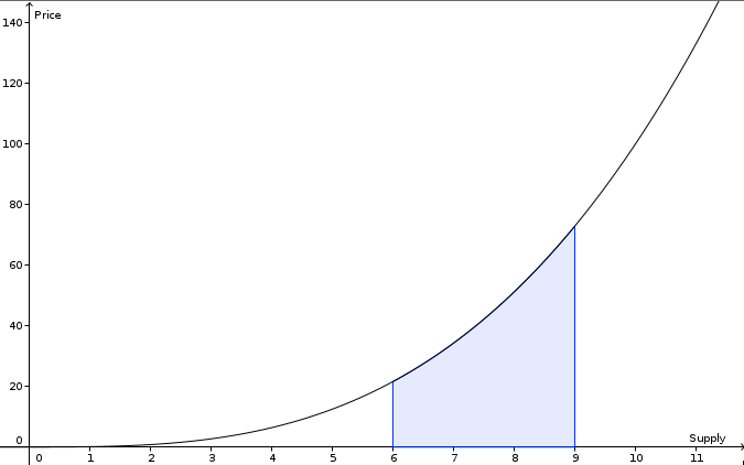
So, finally, what we need to calculate is:

$$p = \int_{s}^{s + k} m \cdot x ^ n = \left\lbrack\frac{m}{n+1}x^{n+1}\right\rbrack_{s}^{s + k} = \frac{m}{n+1}(s+k)^{n+1} - \frac{m}{n+1}s^{n+1}$$

The main problem here are those exponentiations, specially because they could overflow as intermediate results even in perfectly normal scenarios where the final result wouldn’t overflow at all, if the value of n is relatively big. For instance, for n = 10 we would start having problems at about 10M tokens.

We can simplify those formulas, by calculating first the total collateral token staked in the curve (b, for balance), which we can get using the same integral as before but starting at zero and ending at the current bonded token supply, s:

$$b = \frac{m}{n+1} \cdot s^{n+1}$$

Replacing it in the previous formula we get:

$$p = b\left[\left(1 + \frac{k}{s}\right)^{n+1} - 1\right]$$

If we want to sell, we have to repeat the integral above from s to s − k. To get an absolute value instead of a negative number, we also reverse the sign:

$$p = b\left[1 - \left(1 - \frac{k}{s}\right)^{n+1}\right]$$

This is much better for the following reasons:

• What we are exponientating is way lower than before, and it won’t overflow unless the final result does too.
• It’s more intuitive, because now we have b which is the collateral token balance of the curve contract, instead of the more abstract m. Actually to make it even more intuitive we can get rid of n in favour of the reserve ratio, R = 1/(n + 1) and get:

$$p = b\left[1 - \left(1 - \frac{k}{s}\right)^{1/R}\right]$$

So, are we done? Not really, now we have to take the (n+1)-th power of a decimal number… and we only have integers in Solidity.

There’s a bigger issue though. The initial formula above would give us the price p that we need to pay in collateral tokens (ANT) to obtain k bonded tokens (ANJ). But in order to buy we are probably interested in the opposite, i.e. in knowing how much bonded tokens (ANJ) would we get if we deposit p collateral tokens (ANT) into the curve, so we need to isolate k in that equation, and we get:

$$k = s\left[\left(1 + \frac{p}{b}\right)^\frac{1}{n+1} - 1\right]$$

Do you see the problem? Before we needed the n + 1-th power. Letting aside decimals, this is just iterating multiplication. But now we need to calculate the n + 1-th root. We don’t have roots in Solidity at all.

The problem

Our first reaction was to try to fix the issue, as you can see in this repo. The rest of the article explains the approach we took and how we fight the EVM limitations this time.

But before that, let’s explain why we haven’t used it in production yet.

• The explanation by Bancor is fair
• Security and confidence. Bancor contracts had been working on mainnet for long time and, as stated before, the impact of the issue was very low. It would have taken us a lot of time and effort to polish the repo, audit it and make sure it was bullet-proof, for such a sensitive component. You can imagine how bad would a bug in the bonding curve math could be.

We may do this in the future, but at that moment it was not a priority. We still believe that it’s interesting to illustrate the kind of problems you can face when trying to develop smart contracts on Ethereum.

The issue

To overcome this issue of calculating powers and roots, Bancor used a well known technique that consists on using natural logarithms and then exponentiation on base e. So, instead of calculating (1 + k/s)^n + 1 we can do:

e^{(n + 1) ⋅ ln (1 + k/s)}

How the heck can this be any better, you may ask. Well, the thing is that here the base for both the exponentiation and the logarithm are fixed, e, and we can apply tables to get approximations, while before you would have had to pre-compute all the combinations for any base and any exponent. Using tables for computing exponentiations and logarithms was a regular practice only 50 years ago. The blockchain, this technology of the future, brought us back to it.

But the real advantage is for roots, as the exponentiation/logarithm trick turns roots into divisions, so instead of (1 + p/b)^{1/(n + 1)} now we can do:

$$e^{\frac{\ln(1 + p/b)}{n+1}}$$

How those pre-computations in Bancor contracts work is out of the scope of this article, but it’s interesting to understand why the formula reverts for valid inputs. You can read the details in that github issue, but TL;DR: even if we were able to reduce the degrees of freedom to only one for each part of the computation (taking the logarithm and then the exponentiation), we still have infinite values to tabulate. Bancor implementation is dismissing some edge cases to simplify it.

Newton

To overcome the issues we decided instead to keep our journey to the past, over three centuries back, to reach another famous technique: Newton’s method. In particular we use the n-th root algorithm to find the n-th root, by solving the equation x^N = A, which is equivalent to A^1/N (we are only interested in real positive numbers). It is an iterative method, which starts at a hopefully close initial guess, x₀ and then uses the following iteration rule:

$$x_{k+1} = \frac{1}{N} \left[(N-1)x_k + \frac{A}{x_k^{N-1}}\right]$$

So, we need to perform k steps, who knows how many, and in each step a N − 1-th power involving decimal numbers. The solution doesn’t look very promising at first glance…

Initial guess

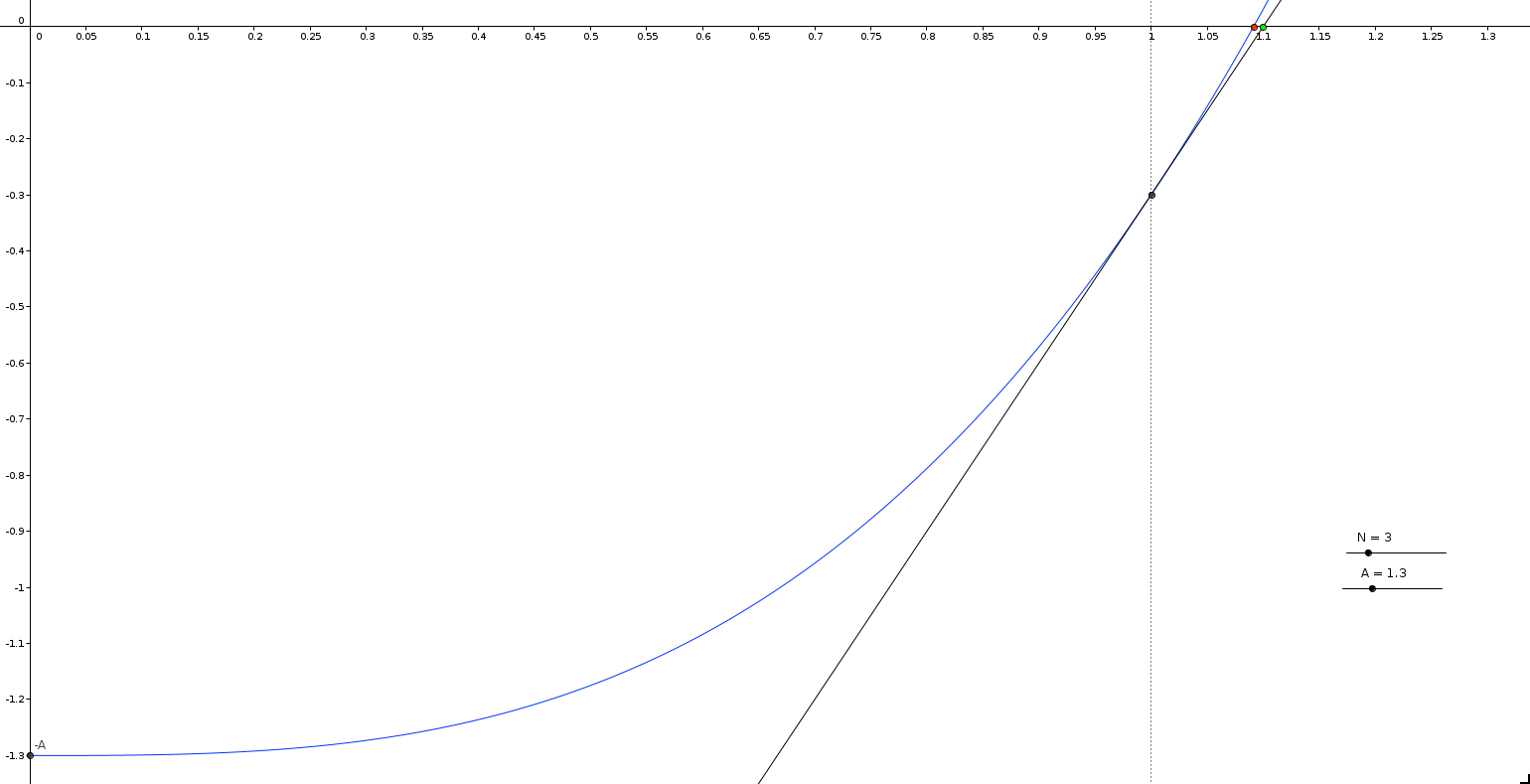
The first approach was to take as initial value the zero of the tangent line to the curve y = x^N − A, which passes by the point (1, 1 − A). This line is always under the curve, as the derivative of that curve is increasing from x = 0 on. Therefore the initial value will always be bigger than the sought value, which seems to behave better for these family of curves. Besides, having x = 1 avoid having to compute powers.

Let’s find that tangent line. First we take the derivative of our curve:

f(x) = x^N − A

f′(x) = N ⋅ x^N − 1

And evaluate on the point we want it to go through, (1, 1), to get the slope of the line, m:

f′(1) = N

We can express our line as:

y − y₀ = m(x − x₀)

Where (x₀, y₀) is our point (1, 1 − A), and m is the slope we just found. Replacing we can arrange it as:

y = Nx − N + 1 − A

Finally we get the zero for that line, and get our initial guess for Newton method:

y = 0

0 = Nx − N + 1 − A

$$x = \frac{A + N - 1}{N}$$

As you can see, it’s just 3 easy operations, and we get a fairly good first approximation (in the figure the ratio between x and y axis is 1:2, so the red and green point are actually closer than it looks) if our base is close to 1, which is probably the most usual case. For instance, a base (A) of 2 would mean that somebody is buying as many tokens as the current total supply, which seems unlikely except during the bootstrapping phase. But even if seldom, it will happen, we can do better.

In the second approach, to make sure that we get very close initial guess, we do the same technique of the tangent line for several growing fixed values.

But as x won’t be 1, the cost of evaluating x^N and x^N − 1 would be significant. To avoid having “hard” computation for that first value, we tabulate them, you can see it in the function _getInitialValue.

The bad news is that in order to get good precision at low computation cost, we need to do it for every possible value of N. You can see that in our repo we have it done up to N = 10. But there’s a script to compute the code for those hardcoded initial values easily.

The contract bytecode size with the current values is around ~15k, so still far from having problems with EIP-170.

Convergence

The function that we are applying Newton Method’s to is f(x) = x^N − A.

Its first derivative is only zero at x = 0 and the second one is always continuous, so having a close enough initial guess ensures the convergence of the method, furthermore, that convergence is quadratic.

Exponentiation

For the “easy” case, the computation of p in the Bancor formula, which only requires the n-th power of those decimal numbers, we use the famous method of exponentiation by squaring.

You can check it out here.

Results

As we wanted, the new version won’t revert unless it really has to: invalid outputs, final result too big, etc. Below you can see how this version compares to original one in terms of precision and gas cost.

As noted by Bancor’s team in their response to the revert issue, “the term optimized by itself has two different interpretations - accuracy & performance - which are typically in “collision” with each other (i.e., improving one hinders the other)”. This is true for our implementation too. In particular, there are two parameters that can be tweaked to modify this trade-off for the root: ROOT_ITERATIONS and ROOT_ERROR_THRESHOLD. The first one defines the largest number of iterations for the Newton method. The second one defines a shortcut for it: if the difference between iterations is less than that threshold, the method will stop.

Precision

To measure precision, we compare values obtained by the original Bancor method and the method proposed in this article, and compare them with the result obtained doing the math in Javascript. So these results must be taken with a grain of salt, as Javascript results have some error too. There’s definitely room for improvement here, but at least we can get a sense of the behaviour of the methods.

• Exponentiation relative error (Sale)

  	Bancor	Simple
  Average	3.924051 %	0.223438 %
  Max	49.748744 %	4.582901 %

• Root relative error (Buy)

  	Bancor	Simple
  Average	1.749319 %	1.753597 %
  Max	49.751238 %	49.751238 %

Gas

As stated above, and as Bancor team explains in the issue, not reverting for those edge cases is not a too much of a benefit. Now that we have checked that our results in terms of precision are good enough, we could ask ourselves what about gas consumption?

• Exponentiation gas used (Sale)

  	Bancor	Simple
  Average	34,418	29,592
  Max	68,591	34,518

• Root gas used (Buy)

  	Bancor	Simple
  Average	33,265	35,365
  Max	57,867	63,099

Conclusion

Some final observations and improvements:

• The method proposed here accomplishes the goal of not reverting without sacrificing precision or gas efficiency. In particular, for exponentiation (sales) it’s considerably better, while for roots (purchases) it’s quite close but slightly worse.
• The revert cases for buying are way more extreme than for selling, so a mixed approach, using the exponentiation by squaring, but avoiding the Newton method for roots, may make sense.
• On one of the non-revert examples, the curve is selling 999 over 1000, and it returns 100 over a balance of 100. So there would be 1 token that would remain stuck. Anyway, I still think it’s better to handle this, reverting if needed, in an upper layer than the math operation.
• Related to the previous one, a nice addition would be to allow to control error direction (floor/ceiling), to make sure it always “benefits the system”.

---